Splice Site Classification
As an example of the PyTorch integration this example will use the UCI Splice-junction Gene Sequences dataset on UCI.
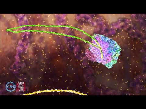
In short, splice sites are locations where the introns and exons connect on pre-mRNA. It's important to understand where these are because the process of splicing removes introns so the exons from the pre-mRNA form mRNA. And mRNA becomes proteins.
Put another way, understanding where the splice sites are helps determine which parts of DNA become proteins.
This is a great 1m37s video from the DNA Learning Center for more context.
From an ML perspective, this is a classification where the sequence is a feature and there is a label, one of:
- Intron to exon (IE) -- Does this sequence contain an intron to exon junction.
- Exon to intron (EI) -- Does this sequence contain an exon to intron junction.
- Neither (N) -- Does this sequence contain neither.
Loading Data
To help load data GCGC contains a FileMetaDataField class that can help turn files into labels.
In this example, the easiest path is to use the SPLICE_DATA_PATH constant, which will point to the
path containing the files EI.fasta, IE.fasta, and N.fasta. The labels for the dataset will become
those files names due to the field.
from gcgc.fields.categorical_field import FileMetaDataField
from gcgc.data import SPLICE_DATA_PATH

files = list(SPLICE_DATA_PATH.glob("*.fasta"))
# [PosixPath('/home/tshauck/gcgc/gcgc/data/splice/EI.fasta'),
#  PosixPath('/home/tshauck/gcgc/gcgc/data/splice/IE.fasta'),
#  PosixPath('/home/tshauck/gcgc/gcgc/data/splice/N.fasta')]
# Each class is a file.

file_feature = FileMetaDataField.from_paths("splice_site", files)
file_feature is one possible features someone might want to model -- in this case the splice
classification. A SequenceParser object can be holds possible features, and in this case the
TorchSequenceParser will go one step further by converting the outputs of the SequenceParser into
native torch objects. See the documentation on sequence parsers for more info.
from gcgc.ml.pytorch_utils.parser import TorchSequenceParser

parser = TorchSequenceParser(file_features=[file_feature])
The SequenceParser can also configure how GCGC will deal with sequences of difference length.
There is one more preparatory step needed before creating the PyTorch compatible Dataset,
and that is to make a GCGC Alphabet. These Alphabet's are subclasses of BioPython Alphabet's class
that support padding, tokenizing and other options relevant for ML applications.
In this case, IUPACAmbiguousDNAEncoding is relevant for DNA with the standard letters plus
extra to deal with ambiguous bases. One example of an ambiguous base letter is that "R" is Purine,
which can be either Adenine ("A") or Guanine ("G").
from gcgc.alphabet import IUPACAmbiguousDNAEncoding

alphabet = IUPACAmbiguousDNAEncoding()
Those ingredients set the stage to create the GenomicDataset object
from gcgc.ml.pytorch_utils.data import GenomicDataset

dataset = GenomicDataset.from_paths(files, parser, alphabet=alphabet)
Given a set of files, from_paths is the best option for generating a GenomicDataset. GCGC uses
BioPython's indexing to work with large files typically found from sequencing samples, and
from_paths will generate the indexes for you with the proper alphabet.
Training
Given the dataset, it's now possible to use PyTorch's built-in DataLoader object which helps with
shuffling, batching, and other common data utilities.
from torch.utils.data import DataLoader

data_loader = DataLoader(dataset, batch_size=128, shuffle=True)
With the data_loader configured we'll create a simple PyTorch model that applies a single 1d convolution layer then a series of dense layers. The output corresponds to the three classes: EI, IE, N.
import torch.nn as nn
import torch.nn.functional as F


class SplicePrediction(nn.Module):
    def __init__(self, vocab_size, num_labels, embed_size=2, num_filters=2, kernel_size=1):
        super().__init__()

        self.embed = nn.Embedding(vocab_size, embed_size)
        self.conv = nn.Conv1d(embed_size, num_filters, kernel_size)

        self.fc1 = nn.Linear(124, 100)
        self.fc2 = nn.Linear(100, 50)
        self.fc3 = nn.Linear(50, num_labels)

    def forward(self, inputs):
        embed = self.embed(inputs).permute(0, 2, 1)

        x = self.conv(embed)
        x = x.view(x.size()[0], -1)
        x = self.fc1(F.relu(x))
        x = self.fc2(F.relu(x))
        x = self.fc3(x)

        return x
Now, it's a matter of training the model by passing it data from the loader. Importantly, the
object iterated through via data_loader has access to a set of keys that are PyTorch tensor
object.
seq_tensor is always present, and represents the input sequence represented as a PyTorch
LongTensor. Also in the example below notice that the splice_site key is present which was the
name of the FileMetaDataField used earlier and represents which class the sequences is a member
of.
import torch

vocab_size = len(alphabet)
num_labels = len(files)
model = SplicePrediction(vocab_size, num_labels)

optimizer = torch.optim.Adam(model.parameters(), lr=0.001)
criterion = torch.nn.CrossEntropyLoss(size_average=False)

model.train()

for i in range(10):  # 10 epochs
    for batch in data_loader:  # Created from the GenomicDataset
        sequences = batch["seq_tensor"].to("cpu")
        target = batch["splice_site"].to("cpu")

        optimizer.zero_grad()
        output = model(sequences)
        loss = criterion(output, target)
        loss.backward()
        optimizer.step()
Because this isn't an example of PyTorch generally, this example doesn't include important considerations like cross-validation, metrics, etc, but hopefully it's clearer how to use GCGC in conjunction with PyTorch.
